How Dumpster Rentals Can Help Your Home Renovation Project
Like a well-oiled machine, a home renovation project requires all its components to function smoothly. One such component, often overlooked, is waste management.
We’re here to discuss how dumpster rentals can be a game-changer for your home renovation project. They’re not just for construction sites; they’re equally beneficial for residential projects too. Dumpster rentals can provide efficient waste management, promote safety, save costs, and help the environment.
Curious about how this unassuming service can pack such a punch in your renovation project? Let’s dive deeper.
Efficient Waste Management With Dumpsters
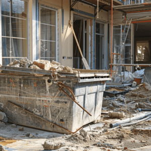
When tackling a home renovation, we can’t overlook the importance of efficient waste management, and that’s where dumpster rentals come into play. These rentals streamline the process of removing waste, accommodating various types of renovation debris in one convenient location. Whether it’s construction waste or discarded materials, a dumpster rental ensures we dispose of everything correctly in one efficient swoop.
Different dumpster sizes are available to suit our project needs and budget constraints. We’re not limited to one size fits all. We can choose a size that’s right for our renovation project, ensuring we’re not paying for space we don’t need or running out of room too quickly.
But it’s not just about the size. Dumpster rental companies provide comprehensive services that save us time and effort. They handle the drop-off, pick-up, and disposal of the waste, so we can focus on the renovation at hand.
Efficient waste management with dumpsters …
- February 28, 2024


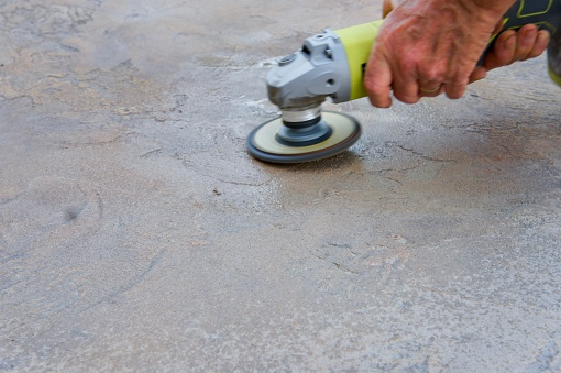
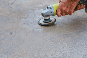 Concrete Grinding is an effective, no-mess, and affordable solution for making your concrete floors and surfaces more slip-resistant and attractive. It’s a very quick way of elevating the aesthetics of any common surface like garage floors, warehouse flooring, pool decks, or even shower stalls! Make your home or business secure and improve your curb appeal with quick and cost-effective concrete floor grinding and polishing.